Tidyverse: A little universe for Analysts

Yes, you heard it right. Tidyverse is a little universe on its own when it comes to data analysis. Let’s explore why it is so.

How does Wikipedia define data analysis?

Data analysis is a process of inspecting, cleansing, transforming, and modeling data to discover useful information, informing conclusions, and supporting decision-making.

In short, if you want to find insights from the data you will use the data analysis process. Now you have got why you use data analysis and it's time to explore how to use it. One of the favorite tools of data analysts is R because it is an open-source and cross-platform, large and welcoming community, high-quality graphics, easy-to-use code and many more.

Tidyverse is a collection of R packages with a common design philosophy for data manipulation, exploration and visualization. That makes tidyverse a good starting point to explore the universe of data.

How to install and load tidyverse in R studio?

To install tidyverse

install.packages("tidyverse")

To load the package in your R environment

library(tidyverse)

Now you are equipped with tidyverse, which means you have installed all the packages in it, lets's see what all things it brings.

Core packages of tidyverse :

• Data Import and management: tibble, readr

• Data Wrangling and Transformation: dplyr ,tidyr ,stringr ,forcats

• Functional Programming: purrr

• Data Visualization and Exploration: ggplot2

Data Import and Management

readr

It provides a fast and friendly way to read rectangular data from delimited files, such as comma-separated values (CSV) and tab-separated values (TSV).To accurately read a dataset with readr, you combine the function with a column specification.

To load readr

library(readr)

import csv file

data <- read_csv("path of your file")

Explore the cheatsheets for readr

tibble

It is a package, which provides opinionated data frames that make working in the tidyverse a little easier. One can say that the tibble package create a simple data frame but with stricter checking and better formatting.

Some of the characteristics of tibbles:

• Never change the datatype of inputs

• Never change the names of variable

• Never create row name

• Make printing easier

To load the package

library(tibble)

Create a tibble from a dataframe

df <- data.frame(a = 1:3, b = letters[1:3], c = Sys.Date() - 1:3)  
as_tibble(df)

// Output
A tibble: 3 x 3
a      b        c         

1     1 a     2022-02-03
2     2 b     2022-02-02
3     3 c     2022-02-01

Create tibble from a dataset e.g. iris dataset

as_tibble(iris)

// Output
A tibble: 150 x 5  
Sepal.Length Sepal.Width Petal.Length Petal.Width Species  
< dbl >     < dbl >      < dbl >     < dbl >      < fct >    
  1          5.1         3.5          1.4         0.2 setosa   
  2          4.9         3            1.4         0.2 setosa   
  3          4.7         3.2          1.3         0.2 setosa   
  4          4.6         3.1          1.5         0.2 setosa   
  5          5           3.6          1.4         0.2 setosa   
  6          5.4         3.9          1.7         0.4 setosa   
  7          4.6         3.4          1.4         0.3 setosa   
  8          5           3.4          1.5         0.2 setosa   
  9          4.4         2.9          1.4         0.2 setosa   
 10          4.9         3.1          1.5         0.1 setosa   
 # ... with 140 more rows

Create a new tibble

tibble(a = 1:3, b = letters\[1:3\], c = Sys.Date() - 1:3)

// Output
A tibble: 3 x 3
  a       b     c         
< int> < chr> < date>    
1       1 a     2022-02-03
2       2 b     2022-02-02
3       3 c     2022-02-01

Data Wrangling and Transformation

dplyr

It contains functions that can perform data manipulation operations such as applying filter, selecting specific column, sorting data, adding or deleting columns and aggregating data. Also these functions are very easy to learn and use.

dplyr Function with their uses:

• select() — to select columns

• filter() — to filter rows.

• group_by() — to group the data

• summarise() — to summarise/aggregate data

• arrange() — to sort the data

• join() — to join data frames (tables)

• mutate() —to create new columns

To load dplyr

library(dplyr)

Use filter function to select rows with Species=setosa and sepal-lenght >5.6

iris %>%   
  filter(.$Species == "setosa" & .$Sepal.Length>5.6)

// Output
Sepal.Length Sepal.Width Petal.Length Petal.Width Species  
1          5.8         4.0          1.2         0.2  setosa  
2          5.7         4.4          1.5         0.4  setosa  
3          5.7         3.8          1.7         0.3  setosa

use mutate fuction to increase the sepal lenght by 0.5

iris %>%   
  head(6) %>%   
  mutate(.$Sepal.Length+0.5)

// Output
Sepal.Length Sepal.Width Petal.Length Petal.Width Species .$Sepal.Length+0.5  
1          5.1         3.5          1.4         0.2  setosa    5.6    
2          4.9         3.0          1.4         0.2  setosa    5.4    
3          4.7         3.2          1.3         0.2  setosa    5.2    
4          4.6         3.1          1.5         0.2  setosa    5.1    
5          5.0         3.6          1.4         0.2  setosa    5.5    
6          5.4         3.9          1.7         0.4  setosa    5.9

tidyr

It is a package that simplifies the process of creating your data tidy. Tabular data is tidy if it is organized in a consistent structure across the dataset and once the data is organized you can move to the further analysis part.

Tidy data standards:

• Variables are organized into columns

• Observations are organized into rows

• Each value must have its own cell

To load tidyr

library(tidyr)

Convert iris dataset from wide to long format

iris %>%   
  pivot_longer(cols=1:4,names_to = "lenght_type",values_to = "lenght")

// Output
A tibble: 600 x 3  
   Species lenght\_type  lenght  
   < fct>  < chr>        < dbl>  
 1 setosa  Sepal.Length    5.1  
 2 setosa  Sepal.Width     3.5  
 3 setosa  Petal.Length    1.4  
 4 setosa  Petal.Width     0.2  
 5 setosa  Sepal.Length    4.9  
 6 setosa  Sepal.Width     3    
 7 setosa  Petal.Length    1.4  
 8 setosa  Petal.Width     0.2  
 9 setosa  Sepal.Length    4.7  
10 setosa  Sepal.Width     3.2  
# ... with 590 more rows

Explore the cheatsheet for tidyr

stringr

The stringr package for string manipulation provides a cohesive set of functions designed to make working with strings as easy as possible. One can say that it is a Simple and Consistent Wrapper for common string operations

To load stringr

library(stringr)

fruit_list=c("apple","banana","orange","grape","mango")

calculate the length of string in a vector :

str_length(fruit_list)

// Output
[1] 5 6 6 5 5

Count the number of vowel present in each fruit name:

str_count(fruit_list,"[aieou]")

// Output
[1] 2 3 3 2 2

join all the fruit name with ',' as a seperator:

str_c(fruit_list,",")

// Output
[1] "apple,"  "banana," "orange," "grape,"  "mango,"

Explore the cheatsheet for stringr

forcats

The forcats package provides a tool for working with factors that are Data structures to store the categorical data in R. The forcats package is to provide a suite of tools that solve common problems with factors, including changing the order of levels or values.

Some of forcats functions are:

• fct_reorder() -  to reorder a factor by another variable

• fct_infreq() - to reorder a factor by frequency of values

• fct_relevel()  - to change the order of factor by hand

To load forcats

install.packages("forcats")

df <- data.frame(A = 1:5, B = letters\[1:5\], C = runif(5,4,12))  
df

// Output
A   B         C  
1  1 a  10.369147  
2  2 b   8.639701  
3  3 c   7.130140  
4  4 d  11.892251  
5  5 e  10.163807

Create a factor

df$A<-factor(df$A)

check the level of factor

levels(df$a)

// Output
[1] "1" "2" "3" "4" "5"

reorder the level of factor using fct_reorder() function

fct_reorder(df$a,df$c)

// Output
[1] 1 2 3 4 5  
Levels: 4 2 5 3 1

Explore the cheatsheet for forcats

Functional Programming

purrr

This package enhances R’s functional programming (FP) toolkit by providing a complete and consistent set of tools for working with functions and vectors. Purrr works with functions and vectors to make your code easier to write and more expressive.

e.g purrr::map() is a function that applies function to each element of a list.

To load purrr

library(purrr)

use purrr function to find squre root of each element in a list

map(c(4,9, 16, 25,30), sqrt)

// Output
[[1]]  
[1] 2  

[[2]]  
[1] 3  

[[3]]  
[1] 4  

[[4]]  
[1] 5  

[[5]]  
[1] 5.477226

Explore the cheatsheat for purrr

ggplot2

It is a plotting package that makes it simple to create complex plots from data in a data frame. It provides a more programmatic interface for specifying what variables to plot, how they are displayed, and general visual properties. ggplot graphics are built step by step by adding new elements as a layer to the existing one providing extensive flexibility and customization of plots.

to load ggplot2

library(ggplot2)

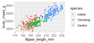
example dataset to show plot

library(palmerpenguins)

plot using scatter points

ggplot(data=penguins)+  
  geom_point(mapping = aes(x=flipper_length_mm,y=body_mass_g,color=species))

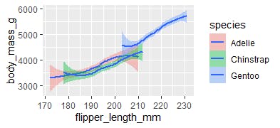
plot using geom smooth

ggplot(data=penguins)+  
    geom_smooth(mapping = aes(x=flipper_length_mm,y=body_mass_g,fill=species))

plot using geom smooth

Explore the cheatsheet for ggplot2

Conclusion

Now that you have got some idea of tidyverse and its capabilities, explore the rest of the little universe ( tidyverse ) and give a boost to your data adventure journey. There are many different packages and tools for data analysis and tidyverse is just one of them so don’t stop here and continue on your learning path.

Hope you enjoyed it!